On this post I will show a mini project I have been working on for the last few days. The goal is generate boolean or binary data from
categorical data. For doing so, I will primarly use Pandas and Numpy libraries. This class was created for testing purposes, so performance has not been taken into account and therefore is not relevant at this moment, however I am convinced that the code can be much more optimized.
Firstly, a short explanation about what this code is doing:
The next table represents the input data, as shown, fields p1, p2, p3 and p4 store categorical data, in this case a product code. Each module consists of four products (p) at most. Note: field "modules" is the index (row names).
| modules |
p1 |
p2 |
p3 |
p4 |
price |
| m_1 |
A1 |
A2 |
|
|
9.90 |
| m_2 |
A1 |
|
A3 |
|
10.50 |
| m_3 |
B1 |
B2 |
A4 |
C1 |
20.30 |
| m_4 |
B1 |
|
A1 |
C1 |
22.10 |
Now, let's imagine we want to solve a linear equation system (Ax = b) composed by field p1, p2, p3 and p4 as matrix "A" , unknows (A1, A2, A3, A4, B1, B2, C1) and price as vector "b":
$A=\begin{bmatrix}a_{11} & a_{12} & \cdots & a_{1n} \\a_{21} & a_{22} & \cdots & a_{2n} \\\vdots & \vdots & \ddots & \vdots \\a_{m1} & a_{m2} & \cdots & a_{mn}\end{bmatrix}, \quad x=\begin{bmatrix}x_1 \\x_2 \\\vdots \\x_n\end{bmatrix}, \quad b=\begin{bmatrix}b_1 \\b_2 \\\vdots \\b_m\end{bmatrix}$
The matrix equations shows that size(A) = m x n, size(x) = n and size(b) = m. On the above example columns(A) is not equal to size(x). Hence, we need a new matrix A with the correct shape, see below.
$A=\begin{bmatrix}1 & 1 & 0 & 0 & 0 & 0 & 0
\\1 & 0 & 1 & 0 & 0 & 0 & 0
\\0 & 0 & 0 & 1 & 1 & 1 & 1
\\1 & 0 & 0 & 0 & 1 & 0 & 1
\end{bmatrix},
\quad x=\begin{bmatrix}A1 \\A2 \\A3 \\A4 \\B1 \\B2 \\C1 \end{bmatrix},
\quad b=\begin{bmatrix}9.90 \\10.50 \\20.30 \\22.10 \end{bmatrix}$
If we get a matrix "A" like the previous one, then we can solve the system easier.
Using vectorial notation, m_1 = A(1, :).x (e.g. Matlab indexing)
Before we continue, I would like to remark that the above system can be easily solvead by isolating x from the equation or by using LU decomposition, especially for square matrices. When dealing with non square matrices ($m \neq n$) the next methods are normaly used:
- Normal equation: $x = (A^{T} A)^{-1} A^{T} b $
- QR factorization
- SVD decomposition
Code:
    import numpy as np
    import pandas as pd
    import warnings
    import matplotlib.pyplot as plt


    class CatBin(object):
        def __init__(self, i_file, o_file=False, cat_cols="all", other_cols=None, op_nan=True):
            """
            Class to convert a matrix with categorical data into a matrix with binary data.

            Example: Convert the below matrix into a binary matrix

                initial_data =
                modules   p1    p2      p3      p4     price
                m_1       A1    A2      nan     nan    9.90
                m_2       A1    nan     A3      nan    10.50
                m_3       B1    B2      A4      C1     20.30
                m_4       B1    nan     A1      C1     22.10

                binary_data =
                modules   A1  A2  A3  A4  B1  B2  C1    price
                m_1       1   1   0   0   0   0   0     9.90
                m_2       1   0   1   0   0   0   0     10.50
                m_3       0   0   0   1   1   1   1     20.30
                m_4       1   0   0   0   1   0   1     22.10

            Uses:
            Solve a linear equation system: Ax = b
                A = matrix[0,1]
                x = [A1, A2, A3, A4, B1, B2, C1]
                b = price

                Note:
                if non-square matrix, we can solve the system by using some
                of the well-known methods:

                    Normal equation
                    QR factorization
                    SVD decomposition

            Graphs - adjacency matrix - connectivity
            ...

            :param i_file: input_file in csv format
            :param o_file: if True a csv is generated. The path must be provided.
            :param cat_cols: slicing - e.g [1, 10] -> from column 1 to 10(not included - pandas)
            :param other_cols:

            if the new data frame must preserve others columns besides those
            with categorical data, position and name should be provided in a dictionary.
                e.g
                others = {'i' : 'modules', 'e', 'prices'}
                if 'i', that column will be inserted on the first position in the new data frame
                    data.insert(0, 'name', column_data)
                if 'e', that column will be inserted after the rest of columns
                    data['name'] = column_data

            :param op_nan: if true all NaN values will be removed.
            """

            self.o_file = o_file
            self.cat_cols = cat_cols
            self.other_cols = other_cols
            self.nan = op_nan
            self.list = []

            self.rows = None
            self.columns = None
            self.p_sparsity = -1

            self.input_data = pd.read_csv(i_file)
            self.boolean_m = None
            self.boolean_a = None

            if self.cat_cols is "all":
                if self.nan is True:
                    # if all data is categorical data to be converted, automatically
                    # others_cols must be false to avoid inconsistencies.

                    self.data = self.input_data.fillna(value='nan')
                else:
                    self.data = self.input_data
                if other_cols is not None:
                    other_cols = None
                    warnings.warn("other_cols has been set to False to avoid inconsistencies")
            else:
                # cat_cols is an array [start, end]
                if isinstance(self.cat_cols, list):
                    if len(self.cat_cols) == 2:
                        _start = self.cat_cols[0]
                        _end = self.cat_cols[1]
                        if self.nan is True:
                            self.data = self.input_data.fillna(value='nan').iloc[:, _start: _end]
                        else:
                            self.data = self.input_data.iloc[:, _start, _end]
                    else:
                        raise ValueError("'start'and 'end' position must be provided")
                else:
                    raise TypeError("cat_cols is not a list")

            if not self.data.empty:
                # extract unique values:
                self.list = self.unique_values()
            else:
                raise ImportError("errors or empty csv file. Check input file")

        def unique_values(self):
            """ return sorted list of unique values """

            u_values = pd.Series(self.data.values.ravel()).unique()
            if self.nan is True:
                return np.sort(u_values[u_values != 'nan'])
            else:
                return np.sort(u_values)

        def boolean_matrix(self):
            matrix = []
            for i in range(len(self.data)):
                v = self.data.iloc[i, :].values
                # avoid worrying about the argument op_nan
                intersect = set(v).intersection(self.list)

                ea = np.zeros(len(self.list))
                for n in intersect:
                    for index, v in enumerate(self.list):
                        if n == v:
                            ea[index] = 1
                matrix.append(ea)

            self.rows = len(matrix)
            self.columns = len(matrix[0])
            self.boolean_m = pd.DataFrame(matrix, columns=self.list)

            return self.boolean_m

        def boolean_augmented_matrix(self):
            """
            The goal of this function is create the augmented matrix:
            Ax = b --> augmented_matrix = [A|b]

            However, this function allows the option of inserting at least
            one first column and many others columns after the boolean data,
            in case that was required to suit your necessities.
            """
            if self.cat_cols is not 'all':
                if self.boolean_m is None:
                    self.boolean_a = self.boolean_matrix()
                else:
                    self.boolean_a = self.boolean_m.copy()

                if self.other_cols is not None and isinstance(self.other_cols, dict):
                    for key, value in self.other_cols.items():
                        if key[0] is 'i':
                            self.boolean_a.insert(0, value, self.input_data[value])
                        elif key[0] is 'e':
                            self.boolean_a[value] = self.input_data[value]
                        else:
                            raise ValueError("Incorrect key format")
                else:
                    warnings.warn("insufficient arguments")
                return self.boolean_a
            else:
                raise ValueError("cat_cols = 'all' the aug. matrix is not possible")

        def sparsity(self):
            """
            The sparsity or density is the fraction of non-zero elements in a matrix.
            :return: ratio non-zero/total
            """
            if self.rows and self.columns and self.boolean_m is not None:
                total = self.rows * self.columns
                non_zeros = sum(self.boolean_m[self.boolean_m == 1].count())
                self.p_sparsity = non_zeros / total
                return "sparsity = {0:.4}%".format(self.p_sparsity * 100)
            else:
                raise ValueError("incorrect data shape. A boolean transformation is required")

        def generate_csv(self, matrix_type='normal'):
            """
            generate a csv file with boolean matrix or augmented matrix
            note: removes first column (index)
            """
            if matrix_type in ['normal', 'augmented']:
                if matrix_type is 'normal':
                    if self.boolean_m is not None:
                        self.boolean_m.to_csv(self.o_file, index=False)
                else:
                    if self.boolean_a is not None:
                        self.boolean_a.to_csv(self.o_file, index=False)
            else:
                raise ValueError("select: normal or augmented")

        @property
        def clean_data(self):
            return self.data

        @property
        def raw_data(self):
            return self.input_data

        @property
        def initial_size(self):
            """ Only includes those fields with categorical data"""
            rows = self.data.shape[0]
            columns = self.data.shape[1]
            return "rows={0}, columns={1}, total={2} elements".\
                format(rows, columns, rows * columns)

        @property
        def final_size(self):
            rows = self.boolean_m.shape[0]
            columns = self.boolean_m.shape[1]
            return "rows={0}, columns={1}, total={2} elements".\
                format(rows, columns, rows * columns)
The code tries to be self-explanatory, however I consider that three functions need more details:
- boolean_matrix: This function contains the basic code to convert the input data. Basically, it compares each row from the initial data "A" with its unique values and inserts one on those positions where matching. As example, this task can be done in Matlab much easier, Matlab can compare two arrays with different length by using the function "ismember()":
          p = {'A1', 'A2', 'A3', 'A4', 'B1', 'B2', 'C1'}; % character arrays or cell arrays
          p_test = {'A1', 'B1','C1'};
          ismember(p, p_test)

          ans =

             1     0     0     0     1     0     1
- boolean_augmented_matrix: The augmented matrix is that obtained by appending the solution vector "b" to matrix "A", usually denoted as [A b] or (A|b). Having a solvable linear equation system, then the augmented matrix [A b] has the same rank as A. Besides of creating the augmented matrix, this function allows the possibility to append other columns if needed.
- Sparsity: The sparsity or density is the fraction of non-zero elements in matrix. A typical example of sparse matrix is the adjacency matrix of an undirected graph.
Below a short example using the class CatBin:
    from others.catbin import CatBin
    import time

    file = "test data/i_simple.csv"
    output_file = "test data/clean_matrix.csv"

    others = {'i': 'modules', 'e': 'price'}

    t1 = time.time()
    ct = CatBin(i_file=file, o_file=output_file, cat_cols=[1, 5], other_cols=others, op_nan=True)

    unique_v = ct.unique_values()
    boolean_m = ct.boolean_matrix()
    boolean_a = ct.boolean_augmented_matrix()
    sparsity = ct.sparsity()
    t = time.time() - t1

    print(t)
    print(ct.initial_size)
    print(ct.final_size)

    ct.generate_csv()
The file "i_simple.csv" is exactly the first table on this post. This code uses all features of the class, producing both boolean matrix and boolean augmented matrix and calculates the sparsity ratio. The most simple example needs 5 lines (without verbose).
    from others.catbin import CatBin

    file = "test data/i_simple.csv"
    output_file = "test data/clean_matrix.csv"

    ct = CatBin(i_file=file, o_file=output_file, cat_cols=[1, 5],
                other_cols={'i': 'modules', 'e': 'price'}, op_nan=True)

    boolean_a = ct.boolean_augmented_matrix()
Results:
      modules  A1  A2  A3  A4  B1  B2  C1  price
    0     m_1   1   1   0   0   0   0   0    9.9
    1     m_2   1   0   1   0   0   0   0   10.5
    2     m_3   0   0   0   1   1   1   1   20.3
    3     m_4   1   0   0   0   1   0   1   22.1

    0.010005950927734375
    rows=4, columns=4, total=16 elements
    rows=4, columns=7, total=28 elements
In my laptop(4GB, i5) the process took 0.01 seconds. The next step will be to test something bigger. The dimensiones of the new data is 2194 x 11:
    1.1577680110931396
    rows=2194, columns=9, total=19746 elements
    rows=2194, columns=294, total=645036 elements
Due to the number of unique values is much higher, the number of elements is almost 650.000 and the process now took 1.15 seconds, surely this can be improved, but for now it works for my purposes. As shown, the new dimensiones will be multiplied by a factor
X(unique values / initial columns).
Hence, having large amount of binary data in a database can also have an impact on performance, so I will not recommend to store the new dataset in a DB better create a system file. There are other options of storing a sparse matrix much more efficient that save the complete data in a DB (CSR or CSC, for instance).
One more example: This dataset includes extra columns before and after the fields with categorical data (2194 x 13). If the order of the extra columns matters is convenient to use ordered dictionaries.
    from others.catbin import CatBin
    from collections import OrderedDict
    import time

    file = "test data/i_data_2.csv"
    output_file = "test data/clean_matrix.csv"

    others = {'i1': 'modules', 'i2': 'modules2', 'e1': 'price', 'e2': 'price2'}
    ordered_others = OrderedDict(sorted(others.items(), key=lambda t: t[0]))

    t1 = time.time()

    ct = CatBin(i_file=file, o_file=output_file, cat_cols=[2, 11],
                other_cols=others, op_nan=True)

    boolean_m = ct.boolean_matrix()
    boolean_a = ct.boolean_augmented_matrix()

    t = time.time() - t1

    sparsity = ct.sparsity()
    print(t)
    print(ct.initial_size)
    print(ct.final_size)
    print(boolean_a)
Finally, a function for plotting:
    def plot_sparse(self, ticks=False, x_ticks=False, y_ticks=False, y_label=None,
                    sparsity=False):
        """
        Notes:
            if sparsity was previously calculated - this figure can be included.
            if data is extraordinarily large might be convenient to hide ticks.
        """
        if sparsity and self.p_sparsity >= 0:
            plt.title("sparsity ratio = {0:.4}%".format(self.p_sparsity * 100), fontsize=10)
            plt.suptitle("boolean matrix", fontsize=14, fontweight='bold')
        else:
            plt.title("boolean matrix", fontsize=14, fontweight='bold')
        plt.imshow(self.boolean_m, interpolation='nearest', cmap='gist_yarg')

        if ticks is True:
            plt.yticks(range(self.boolean_m.shape[0]))
            if x_ticks is True:
                plt.xticks(np.arange(len(self.list)), self.list)
            if y_label is not None and y_ticks is True:
                plt.yticks(np.arange(len(self.input_data[y_label])), self.input_data[y_label])
        else:
            plt.axis('off')

        plt.show()
Let's plot both matrices used on the previous examples:
ct.plot_sparse(ticks=True, x_ticks=True, sparsity=True)
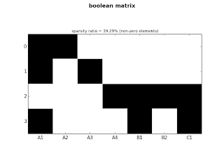 |
| fig.1: small matrix |
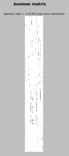
ct.plot_sparse(ticks=False, sparsity=True)
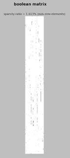 |
| fig.2: medium matrix |
ct.plot_sparse(ticks=True, x_ticks=True, sparsity=True)
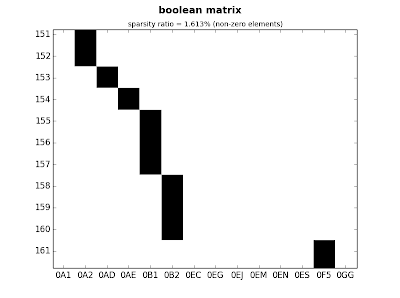 |
| fig.3: medium matrix - detail |
That's all for this post, I hope you find it useful.