Monday, 7 November 2016

Computing the Goodwin-Staton integral

In this post we will explore different approaches for the evaluation of the Goodwin-Staton integral, which is one of the generalizations of the complementary error function. The Goodwin-Staton integral is defined as $$\begin{equation}G(z) = \int_0^{\infty} \frac{e^{-t^2}}{t+z} \; dt \quad |\mathrm{arg}\, z| < \pi \end{equation}$$ From now on, we consider the case where $z$ is real positive number. Note that this special functions can be expressed in terms of other elementary special functions; the error function and the exponential integral. Thus, $$\begin{equation}G(x) = -\frac{e^{-x^2}}{2}(\pi i \mathrm{erf}(ix) + E_i(x^2)) \end{equation}$$ Additionally, the previous representation can be slightly simplified by considering the following connection formulas: $E_i(x) = -E_1(-x)$ and $\mathrm{erfi}(x) = -i\mathrm{erf}(ix)$, where $\mathrm{erfi}(x)$ is the imaginary error function, both valid when $x > 0$. In particular, $E_1(x)$ for real negative argument is not currently supported in Scipy, which will be used for implemented each of the proposed methods.
  from scipy.special import expi, erfi
  from scipy import exp, pi


  def goodwin_staton_1(x):
      mx2 = -x*x
      ans = 0.5 * exp(mx2) * (pi * erfi(x) - expi(-mx2))
      return ans
When $x$ is small the previous equation can be safely evaluated, but for $x \gtrsim 20$ the computation will overflow. This problem is avoidable if we consider some different approaches. A sensible approach consists of substituting the first term using a well-known relation between the imaginary error function and Dawson integral $F(x)$, $$\begin{equation}\frac{\pi \mathrm{erfi}(x)}{2e^{x^2}} = \sqrt{\pi}F(x) \end{equation}$$ On the other hand, the second term involving the exponential integral $E_1(-x^2)$ can be replaced by its asymptotic expansion as follows, $$\begin{equation} \frac{e^{-x^2} E_1(-x^2)}{2} \sim -\frac{1}{2x^2} \sum_{k=0}^{\infty} \frac{k!}{x^{2k}},\quad x \to \infty \end{equation}$$ Therefore, for large argument the Goodwin-Staton integral can be computed as $$\begin{equation} G(x) \sim \sqrt{\pi} F(x) -\frac{1}{2x^2} \sum_{k=0}^{\infty} \frac{k!}{x^{2k}},\quad x \to \infty \end{equation}$$
  from scipy.special import dawsn
  from scipy import pi, exp, sqrt


  def goodwin_staton_2(x):
      # compute Dawson's integral
      term1 = sqrt(pi) * dawsn(x)

      # compute series
      maxiter = 1000
      eps = 2.2e-16
      acc = False
      s = 1.0
      sp = s
      n = 1
      d = 1
      x2 = x*x

      for k in range(1, maxiter):
          n *= k
          d *= x2
          s += n / d
          if abs((s - sp) / sp) < eps:
              if acc:
                  break
              else:
                  acc = True
          else:
              sp = s

      ans = term1 - 0.5 * s / x2
      return ans
Another alternative is representing the second term as definite integral, $$\begin{equation} \frac{e^{-x^2} E_1(-x^2)}{2} = - \frac{1}{2}\int_0^1 \frac{dt}{x^2 + \log(t)} \end{equation}$$ Therefore, the Goodwin-Station is represented as follows, $$\begin{equation} G(x) = \sqrt{\pi}F(x) - \frac{1}{2}\int_0^1 \frac{dt} {x^2 + \log(t)} \end{equation}$$
from scipy.integrate import quad
from scipy.special import dawsn
from scipy import log, inf, sqrt, pi


def integrand(t, x):
    return 1 / (x * x + log(t))


def term2_integral(x):
    eps = 2.2e-16
    return quad(integrand, 0, 1, args=x, epsabs=eps, epsrel=eps, limit=100)


def goodwin_staton_3(x):
    # compute Dawson's integral
    term1 = sqrt(pi) * dawsn(x)

    # compute integral
    term2, err = term2_integral(x)

    return term1 - 0.5 * term2, err
Finally, we can evaluate the integral using an adaptive quadrature algorithm implemented in scipy.integrate.quad, based on the Fortran library QUADPACK.
from scipy.integrate import quad
from scipy import exp, inf


def integrand(t, x):
    return exp(-t**2) / (t + x)


def goodwin_staton_4(x):
    eps = 2.2e-16
    return quad(integrand, 0, inf, args=x, epsabs=eps, epsrel=eps, limit=100)
In order to perform a check of correctness, we evaluate the integral definition using the tanh-sinh or double exponential integration algorithm implemented in mpmath with 20 digits of precision. For example,
>>> from mpmath import *
>>> mp.dps = 20
>>> z = 10
>>> quad(lambda t: exp(-t*t)/(t + z), [0, inf])
mpf('0.084021593706602168771586')

Wednesday, 1 July 2015

Interior Point Method: Primal Affine scaling algorithm in Python

On this post we implement The Primal Affine scaling algorithm, one of the Interior Point Methods. Let us start by the Problem Formulation:


$\begin{equation*}\label{a} \begin{aligned} & {\underset{x} min} & & c^T x\\ & \text{subject to} & & Ax= b \quad \quad \quad (P)\\ &&& x \ge 0\\ \end{aligned} \end{equation*}$

where $x\in \mathbb{R}^n$ is the vector of variables, $c \in \mathbb{R}^n$ is the vector of linear costs, $A \in \mathbb{R}^{m\times n}$ is the matrix of constraint and $b \in \mathbb{R}^m$ is the right-hand-side vector. In general, two main hypothesis are considered: Matrix $A$ is full row rank and $P$ is nondegenerate. However, as shown later, some techniques are available to deal with problems where $A$ is not full rank.

This algorithm includes a Big-M formulation and therefore the Big-M value must be chosen in advance, several approaches are possible:
A first approach is start $M$ with a large value, $10^{30}$, for instance. However, if $M$ is too large it can causes numerical problems, since it is known that the presence of coefficients larger than the rest of variables by many orders of magnitude have potentially undesirable numerical aspects. Therefore, ideally we should search for a $\textit{"sufficiently large"}$ $M$. A standard decision is choose a $M$ value which is at least $n$ times larger than the largest value of any of the variables in the specific Linear programming problem.
For this implementation, the second approach with $n=100$ was chosen. Nevertheless, the first approach has been also tested, obtaining bad results in several problems, with numerical instability when approaching to the optimal value, hence,

$\begin{equation}\label{big-m} M = n \cdot \mathrm{max}_{1 \le i \le n}\;|c_i| \end{equation}$

where $c$ is the cost vector and $n$ the number of variables. In any case, the presented implementation provides the option of supplying a custom $M$ in case the user previously knows an upper or lower bound on some quantity (e.g. a capacity limit).

We focus now on the algorithm implementation. The primal affine scaling algorithm has been implemented in a class called PrimalAffine() with several arguments. Furthermore, a function called _pre_check checks the input of the class: If the matrix and vectors are of the class ndarray. A relevant function is _check: This function validates that the vector $b$ and $c$ are column vectors and checks if the matrix $A$ is a full matrix, otherwise throw an exception and do not continue solving the problem. This check can be removed if the Cholesky decomposition for semidefinite matrices is implemented (we implement it later).

The following code is the main routine in the algorithm, where two functions $({\tt \_dual\_gap}$ and ${\tt \_compute\_y})$ are included. Basically, these two separated functions aim to improve readability.
import numpy as np
import scipy.io
from scipy.sparse import csr_matrix
import scipy
import pandas as pd
import time
import matplotlib.pyplot as plt
import math
import numba


class PrimalAffine(object):
    def __init__(self, c, a, b, opt_gap=1.0e-6, eps=1.0e-12, rho=0.95, m=None):
        self.c = c
        self.a = a
        self.b = b
        self.opt_gap = opt_gap
        self.eps = eps
        self.rho = rho
        self._alphas = []
        self._f_values = []
        self._gaps = []
        self._iter = []
        self._pre_check()

        if m is None:
            self.m = 100 * np.max(abs(self.c))
        else:
            self.m = m
        print("Max value = {}".format(np.max(abs(self.c))))
        print("Big-M = {}".format(self.m))

        self._optimize_primal()

    def _pre_check(self):
        if not (isinstance(self.a, np.ndarray) or isinstance(self.b, np.ndarray) or isinstance(self.c, np.ndarray)):
            raise Exception('Inputs must be a numpy arrays')

    def _check(self, ra, ca, rb, rc):
        if np.linalg.matrix_rank(self.a) != ra:
            raise Exception('Matrix A is not full rank')

        if rb != ra:
            if np.size(self.b) == ra:
                self.b = np.transpose(self.b)
            else:
                raise AttributeError('dimension of vector b is not correct')

        if rc != ca:
            if np.size(self.c) == ca:
                self.c = np.transpose(self.c)
            else:
                raise AttributeError('dimension of vector b is not correct')

    def _optimize_primal(self):

        r_a, c_a = np.shape(self.a)
        r_b = np.shape(self.b)[0]
        r_c = np.shape(self.c)[0]

        self._check(r_a, c_a, r_b, r_c)

        x = np.ones((c_a, 1))
        a = np.c_[self.a, self.b - np.dot(self.a, x)]
        x = np.ones((c_a + 1, 1))
        c = np.vstack([self.c, self.m])
        d = np.eye(c_a + 1)
        y = self._compute_y(a, d, c)

        i = 0
        while self._dual_gap(c, x, self.b, y) > self.opt_gap:
            z = c - np.dot(np.transpose(a), y)
            dx = np.dot(-d, z)
            if np.all(dx >= 0):
                print('Unbounded problem')
                break
            alpha = self.rho * np.min(-x[dx < self.eps] / dx[dx < self.eps].ravel())
            x += alpha*dx
            d = np.diag(x.ravel())**2
            y = self._compute_y(a, d, c)
            i += 1

            f_obj = np.dot(np.transpose(c), x)
            self._f_values.append(f_obj.ravel()[0])
            self._alphas.append(alpha.ravel()[0])
            self._gaps.append(self._dual_gap(c, x, self.b, y).ravel()[0])

        if x[c_a] > 1e-5:
            print('Infeasible problem. x[n+1] = {}'.format(x[c_a]))
        else:
            pass
            print('\n', x[0:c_a])

    def _compute_y(self, aa, dd, cc):
        term1 = np.dot(np.dot(aa, dd), np.transpose(aa))
        term2 = np.dot(np.dot(aa, dd), cc)
        L = self._chol_semidefinite(term1)
        sol = self._chol_solve(L, term2)
        return sol

    @staticmethod
    def _dual_gap(cc, xx, bb, yy):
        term1 = np.dot(np.transpose(cc), xx)
        term2 = term1 - np.dot(np.transpose(bb), yy)
        term3 = 1.0 + abs(term1)
        return abs(term2)/term3

    @staticmethod
    @numba.autojit
    def _chol_semidefinite(A):
        n = len(A)

        # create zero matrix for L
        L = np.zeros((n, n))

        # Perform the Cholesky decomposition
        for i in range(n):
            for k in range(i+1):
                tmp_sum = 0
                for j in range(k):
                    tmp_sum += L[i, j] * L[k, j]

                if i == k:  # diagonal
                    L[i, k] = math.sqrt(A[i, i] - tmp_sum)
                    if L[i, k] <= 0:
                        L[i, k] = 10**10

                else:
                    L[i, k] = (1.0 / L[k, k] * (A[i, k] - tmp_sum))
        return L

    @staticmethod
    def _chol_solve(L, b):
        L_inv = np.linalg.inv(L)
        z = np.dot(L_inv, b)
        y = np.dot(np.transpose(L_inv), z)
        return y


    def results(self):
        d = {'gap': self._gaps, 'fobj': self._f_values, 'alpha': self._alphas}
        df = pd.DataFrame(d)
        print(df)
A few comments about the above code:
  • An important point is to check whether the problem is infeasible or not. Therefore, if $x_{n+1}^* > \epsilon_{inf}$ then problem $(P)$ is infeasible, due to $M \gg 0$ in the optimal solution and hence, $x_{n+1}^* \approx 0$. We set $\epsilon_{inf}$ to $1{e-}5$.
  • We included the function to compute the Cholesky decomposition in a positive semidefinite matrix. Unfortunately, this implementation is not very efficient, even using good libraries like ${\tt Numpy}$, so in order to speed up the computation we use the library ${\tt Numba}$ so that the code can be just-in-time compiled by using the LLVM compiler. The ${\tt @numba.autojit}$ decorator tells ${\tt Numba}$ to compile the function. In average, by using a JIT compiler, it is possible to achieve $\times 3$ speed up. This function is based on the Cholesky-Banachiewicz algorithm applying a modification, so that if a value of the diagonal is 0 (zero pivot), it is replaced by a large value $L_{ik} = 10^{64}$ that is in a sense surrogates for $\infty$.
Furthermore, we can test our algorithm solving problems of the Netlib collection. The Netlib problems in format ${\tt .mat}$ have been downloaded from NETLIB problems. As the algorithm was implemented in Python a function has been included to read .mat files.
def mat_parse(file):
    mat_content = scipy.io.loadmat(file)
    mat_struct = mat_content['Problem']
    val = mat_struct[0, 0]
    A = csr_matrix(val['A']).todense()
    b = val['b']
    c = val['aux'][0][0][0]
    return A, b, c


if __name__ == '__main__':
    # http://www.cise.ufl.edu/research/sparse/mat/LPnetlib/
    A, b, c = mat_parse('lp_sctap3.mat')

    print(np.shape(A))
    print(np.shape(b))
    print(np.shape(c))

    t1 = time.perf_counter()
    primal = PrimalAffine(c, A, b, opt_gap=1e-6)
    elapsed = (time.perf_counter() - t1)
    print(elapsed)
    primal.results()
Finally, this is a small example that shows the behaviour of this algorithm:
$\begin{equation} A = \begin{pmatrix} 2 & 1 & -1 & 0\\ 3& 4& 0 & 1\\ \end{pmatrix} \quad b = \begin{pmatrix} 2 \\ 12 \end{pmatrix} \quad c=\begin{pmatrix} 3 \\ 1 \\ 0 \\ 0 \end{pmatrix} \end{equation}$
And the following table and plot summarize the steps towards the optimal solution of the problem:

 
Iter alpha fobj gap x1 x2 x3 x4
0 0.0086 19.52871 0.76302 0.85813 1.95431 1.67057 1.40837
1 0.0636 5.15115 0.35592 0.78414 2.04874 1.61701 1.44264
2 0.7896 2.96509 0.08685 0.03921 2.54061 0.61903 1.71583
3 3.1027 2.27926 0.06842 0.03034 2.17289 0.23358 3.2172
4 4.4464 2.05176 0.01697 0.02578 1.96012 0.01168 4.082
5 36.9018 2.01468 0.00486 0.00129 2.00406 0.00664 3.97979
6 140.6546 2.00183 0.00061 0.00106 1.99833 0.00044 4.00352
7 900.1966 2.00055 0.00018 0.00005 2.00016 0.00027 3.9992
8 3579.9455 2.00009 0.00003 0.00004 1.99993 0.00001 4.00016
9 22196.8995 2.00002 0.00001 0 2.00001 0.00001 3.99997
10 101489.1179 2 0 0 2 0 4.00001
11 425757.3225 2 0 0 2 0 4
 
Figure 1: Steps towards the optimal solution. Optimal solution = 2. x1 = 0 and x2 = 2. Total number of iterations = 12.

Friday, 24 April 2015

AMPL reporting solver statistics

This a simple script that I have been working on, which provides some Solver statistics to AMPL. At this moment, the script can handle the MINOS solver output and generate cool charts to summarize the process till the solver reaches a solution.
As usual, I have written a python script that is called by the shell command in AMPL.

option solver minos;
option minos_options "Superbasics_limit=100 summary_file=1 1=summary.txt summary_level = 1 summary_frequency=1";
  
printf "MINOS_report: generating AMPL results...\n";
shell 'C:\Python27\python.exe "MINOS_report.py" summary.txt';
As said, this script was written to work with MINOS, so after choosing MINOS as solver, we must provide to MINOS the output file which will contain the solver's statistics. The python script just parse the output file, clean it and generate the chart shown below. This code is just an example and does not aim to be very fast or optimum in terms of computational efficiency since is just a first test.
import pandas as pd
import matplotlib.pyplot as plt
import sys
import os


class Generate(object):
    def __init__(self, i_file):
        self.f_input = i_file
        self.f_output = "results_clean.csv"
        self.data = []
        self.output = []

    def clean_file(self):
        with open(self.f_input, "r") as f:
            it = 0
            for line in f:
                if "EXIT" in line:
                    break
                elif line[:7].strip().isdigit() and int(line[:7].strip()) > it \
                        and not "T" in line:
                    if len(line) > 10:
                        #print line
                        it += 1
                        self.output.append(line)
        f.close()
        w = open(self.f_output, "w")
        w.writelines(self.output)
        w.close()
        print "MINOS_report: new file > {0}".format(self.f_output)

    def get_data(self):
        cols = [(1, 7), (8, 16), (17, 22), (23, 32), (33, 48), (49, 54), (55, 60), (61, 65)]
        self.data = pd.read_fwf(self.f_output, colspecs=cols, header=None)

    def plots(self):

        itn = len(self.data)
        rgradient = self.data[1]
        ninf = self.data[2]
        sinf = self.data[3]
        objective = self.data[4]
        nobj = self.data[5]
        ncon = self.data[6]
        nsb = self.data[7]

        it = list(range(1, itn + 1))

        _min_obj = objective[itn - 1]
        _max_nsb = nsb[itn - 1]
        _max_nobj = nobj[itn - 1]
        _sinf = sinf[itn - 1]
        _ninf = ninf[itn - 1]
        _ncon = ncon[itn - 1]

        plt.figure("AMPL results")

        # plot 1
        # ~~~~~~~~~~~~~~~~~~~~~~~~~~~~~~~~~~~~~~~~~~~~~~~~~~~~~~~~~~~~~~~~~~~~~~~~~~~~~~~~~~
        ax1 = plt.subplot(211)
        ax1.set_title('Iterations={0}. Objective (optimal solution)={1}'
                      .format(itn, _min_obj), size=10)

        ax1.set_xlabel('iterations')
        ax1.set_ylabel('objective function')
        l_obj = ax1.plot(it, objective, '.-', color="#0E3EEB", label="obj")
        ax2 = ax1.twinx()
        ax2.set_ylabel('reduced gradient')
        l_rg = ax2.plot(it, rgradient, '.-', color="#EB710E", label="rg")

        lns = l_obj + l_rg
        labs = [l.get_label() for l in lns]

        ax1.grid()
        ax1.legend(lns, labs, loc=0)

        # plot 2
        # ~~~~~~~~~~~~~~~~~~~~~~~~~~~~~~~~~~~~~~~~~~~~~~~~~~~~~~~~~~~~~~~~~~~~~~~~~~~~~~~~~~
        ax3 = plt.subplot(223)
        ax3.set_title('number of superbasics={0}\n # objective and gradient calculations={1}'
                      .format(_max_nsb, _max_nobj), size=10)

        l_sb = ax3.plot(it, nsb, '.-', color="#0E3EEB", label="nsb")
        ax3.set_xlabel('iterations')
        ax3.set_ylabel('no.superbasics')
        ax4 = ax3.twinx()
        l_nobj = ax4.plot(it, nobj, '.-', color="#EB710E", label="nobj")
        ax4.set_ylabel('calculations obj. & gradient')

        lns = l_sb + l_nobj
        labs = [l.get_label() for l in lns]

        ax3.grid()
        ax3.legend(lns, labs, loc=4)

        # plot 3
        # ~~~~~~~~~~~~~~~~~~~~~~~~~~~~~~~~~~~~~~~~~~~~~~~~~~~~~~~~~~~~~~~~~~~~~~~~~~~~~~~~~~
        plt.subplot(224)
        plt.title('no. of infeasibilities={0}\n sum of infeasibilities={1}\n '
        '# nonlinear constraints evaluations={2}'.format(_ninf, _sinf, _ncon), size=10)
        plt.plot(it, ncon, 'g-', label="ncon")
        plt.plot(it, ninf, 'y-', label="ninf")
        plt.plot(it, sinf, 'm-', label="sinf")
        plt.xlabel('iterations')
        plt.grid()
        plt.legend()

        plt.tight_layout()
        plt.show()


if __name__ == "__main__":
    summary_file = sys.argv[1]
    #summary_file = "C:/Users/Guillermo Navas/Desktop/MSc Statistics and Operations research/Continuous optimization/" \
    #                   "Modelling and solving optimization problems/Lab assignment 2 _ Network flow problems/solver_summary.txt"
    report = Generate(summary_file)
    report.clean_file()
    report.get_data()
    report.plots()

Friday, 31 October 2014

creating shared library AMPL

On this post I will try to explain in detail how create a shared library for AMPL. At this moment the Extended Function Library extends AMPL with over 300 functions, all of them available on the GNU Scientific library. Hence, before creating your own library you should check if your function is already included in that library.

I started my custom library because I needed the sigmoid function for one project and that function was not available in the Extended Function Library.

This process has the next steps:

  • Download headers: funcadd.h and stdio.1.h
  • Visual Studio: create a new Win32 project -> DLL.
  • Build DLL and testing.

The headers can be downloaded from the pages below:

Once this is done, create a new project -> Win32 project in Visual Studio and select application type DLL. Add both headers to Header Files and create a new file for your functions (e.g mathFuncs.c). Now your solution explorer should look like this:

Figure 1. Solution Explorer - Visual Studio

As said, we will create the sigmoid function and an approximation, the C code below shows one possible implementation, surely can be improved to gain efficiency. But before getting into the code, let's explain some general concepts about solvers and sigmoid functions. In general, the solvers need the first and second order derivatives of the function, depending on the method implemented by the solver (quasi-newton, newton's method, etc.), they may require the first derivative or both, as example MINOS requires just the first order derivative since it approximates the second one. In this .dll we will provide both derivatives of the functions.

Sigmoid function: $\frac{1}{(1 +\exp(-x))}$

First order derivative: $\frac{1}{(1 +\exp(-x))} (1 - \frac{1}{(1 +\exp(-x))}) = sigmoid(x)(1-sigmoid(x))$

Second order derivative: $\frac{-(\exp(x)(\exp(x) - 1))}{(\exp(x) + 1)^3}$

A possible sigmoid function approximation ,computationally faster, is the "fast sigmoid" function. The evaluation of the exponential function has a relevant cost and in many situations the exact sigmoid function may not be needed. This post is an interesting resource about the topic with a good benchmarking between methods link.

Fast sigmoid function: $\frac{x}{(1 + |x|)}$

First order derivative: $\frac{(-\frac{x^2}{|x|} + |x| + 1)}{|x|(1 + |x|)^2}$

Second order derivative: $\frac{3x^2|x| - 3|x|^3 - 3|x|^2 + x^2}{|x|^3(|x| + 1)^3}$

#include "stdlib.h"
#include "math.h"
#include "funcadd.h"    /* includes "stdio1.h" */

#define MAX_VAL 1.0e+300

#ifdef __cplusplus
/* The #ifdef __cplusplus lines allow this to be compiled
 * either by an ANSI C compiler or by a C++ compiler.
 */
extern "C" {
#endif

 static real
sigmoid(arglist *al)
 {
     /*  Sigmoid function: sigmoid(x) = 1/(1 + exp(-x)) */
     
     real x = al->ra[0];
     AmplExports *ae = al->AE;

     if (x > MAX_VAL || x < -MAX_VAL) 
     {
         fprintf(Stderr, "x = %d exceeded the maximum allowed value.", x);
         return -1;
     }
     else
     {
        if (al->derivs)
        {
            //first derivative: sigmoid gradient
            //  domain: R (all real numbers)
            //  range: {y c R: 0 <= y <= 0.25}

            *al->derivs = (1.0f/(1.0f + exp(-x)))*(1.0f -1.0f/(1.0f + exp(-x)));
            if (al -> hes)
            {
                //second derivative (hessian)
                //  domain: R (all real numbers)
                //  range: {y c R: -1/(6*sqrt(3)) <= 1/(6*sqrt(3))}

                *al->hes = -(exp(x) * (exp(x) - 1.0f)/ (pow(exp(x) + 1.0f, 3)));
            }
        }
        return 1.0f/(1.0f + exp(-x));
     }   
 }
 
 static real
fast_sigmoid(arglist * al)
 {
    /* fast sigmoid: sigmoid function approximation.
       fast_sigmoid(x) = x/(1 + abs(x))

       Domain {x c R: x != 0} -> derivative discontinuity at x = 0
     */
     
     real x = al->ra[0];
     if (al->derivs)
     {
         // first derivative (gradient)
         *al->derivs = (-pow(x,2)/fabs(x) + fabs(x) + 1) /(fabs(x) * pow(1 + fabs(x), 2));
         
         if (al -> hes)
         {
             // second derivative (hessian)
             real d = 3 * pow(x,2) * fabs(x) - 3 * pow(fabs(x), 3);
             real d1 = 3 * pow(fabs(x),2) + pow(x,2);
             *al->hes = (d  - d1) / (pow(fabs(x), 3) * pow(fabs(x) + 1, 3));
         }
     }
     return x / (1 + fabs(x));  
 }

 void
funcadd(AmplExports *ae){
/* Insert calls on addfunc here... */

/* Arg 3, called type, must satisfy 0 <= type <= 6:
 * type&1 == 0: 0,2,4,6 ==> force all arguments to be numeric.
 * type&1 == 1: 1,3,5   ==> pass both symbolic and numeric arguments.
 * type&6 == 0: 0,1 ==> the function is real valued.
 * type&6 == 2: 2,3 ==> the function is char * valued; static storage
                suffices: AMPL copies the return value.
 * type&6 == 4: 4,5 ==> the function is random (real valued).
 * type&6 == 6: 6   ==> random, real valued, pass nargs real args,
 *              0 <= nargs <= 2.
 *
 * Arg 4, called nargs, is interpretted as follows:
 *  >=  0 ==> the function has exactly nargs arguments
 *  <= -1 ==> the function has >= -(nargs+1) arguments.
 */

    addfunc("sigmoid", (rfunc) sigmoid, 0, 1, 0);
    addfunc("f_sigmoid", (rfunc) fast_sigmoid, 0, 1, 0);
}

#ifdef __cplusplus
    }
#endif

When creating a custom functions there are two important points, write the first order derivative (*al ->derivs) and if there is second derivative (if the solver's method requires the second order derivative for computing the Hessian ; al -> hes) then (*al->hes).

A last comment regarding funcadd(); It is important to define appropiate names to call your function (first argument in addfunc()), in this case I chose "sigmoid" and "f_sigmoid", keep in mind this, because otherwise AMPL will not recognize your functions.

Now it is time to build the .dll and do some testing with AMPL. Paste your .dll into your AMPL directory:

Figure 2. AMPL directory (student-edition)
Open ampl.exe or amplide.exe and type the instructions below to test your functions; if you followed these steps your output should be identical.
Figure 3. AMPL console
That's all from my side, I hope you find it useful.

Thursday, 14 August 2014

Sparse matrix: from categorical matrix to binary matrix

On this post I will show a mini project I have been working on for the last few days. The goal is generate boolean or binary data from categorical data. For doing so, I will primarly use Pandas and Numpy libraries. This class was created for testing purposes, so performance has not been taken into account and therefore is not relevant at this moment, however I am convinced that the code can be much more optimized.

Firstly, a short explanation about what this code is doing:

The next table represents the input data, as shown, fields p1, p2, p3 and p4 store categorical data, in this case a product code. Each module consists of four products (p) at most. Note: field "modules" is the index (row names).

modules p1 p2 p3 p4 price
m_1 A1 A2 9.90
m_2 A1 A3 10.50
m_3 B1 B2 A4 C1 20.30
m_4 B1 A1 C1 22.10

Now, let's imagine we want to solve a linear equation system (Ax = b) composed by field p1, p2, p3 and p4 as matrix "A" , unknows (A1, A2, A3, A4, B1, B2, C1) and price as vector "b":

$A=\begin{bmatrix}a_{11} & a_{12} & \cdots & a_{1n} \\a_{21} & a_{22} & \cdots & a_{2n} \\\vdots & \vdots & \ddots & \vdots \\a_{m1} & a_{m2} & \cdots & a_{mn}\end{bmatrix}, \quad x=\begin{bmatrix}x_1 \\x_2 \\\vdots \\x_n\end{bmatrix}, \quad b=\begin{bmatrix}b_1 \\b_2 \\\vdots \\b_m\end{bmatrix}$

The matrix equations shows that size(A) = m x n, size(x) = n and size(b) = m. On the above example columns(A) is not equal to size(x). Hence, we need a new matrix A with the correct shape, see below.

$A=\begin{bmatrix}1 & 1 & 0 & 0 & 0 & 0 & 0 \\1 & 0 & 1 & 0 & 0 & 0 & 0 \\0 & 0 & 0 & 1 & 1 & 1 & 1 \\1 & 0 & 0 & 0 & 1 & 0 & 1 \end{bmatrix}, \quad x=\begin{bmatrix}A1 \\A2 \\A3 \\A4 \\B1 \\B2 \\C1 \end{bmatrix}, \quad b=\begin{bmatrix}9.90 \\10.50 \\20.30 \\22.10 \end{bmatrix}$

If we get a matrix "A" like the previous one, then we can solve the system easier.
Using vectorial notation, m_1 = A(1, :).x (e.g. Matlab indexing)

Before we continue, I would like to remark that the above system can be easily solvead by isolating x from the equation or by using LU decomposition, especially for square matrices. When dealing with non square matrices ($m \neq n$) the next methods are normaly used:

  • Normal equation: $x = (A^{T} A)^{-1} A^{T} b $
  • QR factorization
  • SVD decomposition

Code:

    import numpy as np
    import pandas as pd
    import warnings
    import matplotlib.pyplot as plt


    class CatBin(object):
        def __init__(self, i_file, o_file=False, cat_cols="all", other_cols=None, op_nan=True):
            """
            Class to convert a matrix with categorical data into a matrix with binary data.

            Example: Convert the below matrix into a binary matrix

                initial_data =
                modules   p1    p2      p3      p4     price
                m_1       A1    A2      nan     nan    9.90
                m_2       A1    nan     A3      nan    10.50
                m_3       B1    B2      A4      C1     20.30
                m_4       B1    nan     A1      C1     22.10

                binary_data =
                modules   A1  A2  A3  A4  B1  B2  C1    price
                m_1       1   1   0   0   0   0   0     9.90
                m_2       1   0   1   0   0   0   0     10.50
                m_3       0   0   0   1   1   1   1     20.30
                m_4       1   0   0   0   1   0   1     22.10

            Uses:
            Solve a linear equation system: Ax = b
                A = matrix[0,1]
                x = [A1, A2, A3, A4, B1, B2, C1]
                b = price

                Note:
                if non-square matrix, we can solve the system by using some 
                of the well-known methods:

                    Normal equation
                    QR factorization
                    SVD decomposition

            Graphs - adjacency matrix - connectivity
            ...

            :param i_file: input_file in csv format
            :param o_file: if True a csv is generated. The path must be provided.
            :param cat_cols: slicing - e.g [1, 10] -> from column 1 to 10(not included - pandas)
            :param other_cols:

            if the new data frame must preserve others columns besides those
            with categorical data, position and name should be provided in a dictionary.
                e.g
                others = {'i' : 'modules', 'e', 'prices'}
                if 'i', that column will be inserted on the first position in the new data frame
                    data.insert(0, 'name', column_data)
                if 'e', that column will be inserted after the rest of columns
                    data['name'] = column_data

            :param op_nan: if true all NaN values will be removed.
            """

            self.o_file = o_file
            self.cat_cols = cat_cols
            self.other_cols = other_cols
            self.nan = op_nan
            self.list = []

            self.rows = None
            self.columns = None
            self.p_sparsity = -1

            self.input_data = pd.read_csv(i_file)
            self.boolean_m = None
            self.boolean_a = None

            if self.cat_cols is "all":
                if self.nan is True:
                    # if all data is categorical data to be converted, automatically 
                    # others_cols must be false to avoid inconsistencies.
                    
                    self.data = self.input_data.fillna(value='nan')
                else:
                    self.data = self.input_data
                if other_cols is not None:
                    other_cols = None
                    warnings.warn("other_cols has been set to False to avoid inconsistencies")
            else:
                # cat_cols is an array [start, end]
                if isinstance(self.cat_cols, list):
                    if len(self.cat_cols) == 2:
                        _start = self.cat_cols[0]
                        _end = self.cat_cols[1]
                        if self.nan is True:
                            self.data = self.input_data.fillna(value='nan').iloc[:, _start: _end]
                        else:
                            self.data = self.input_data.iloc[:, _start, _end]
                    else:
                        raise ValueError("'start'and 'end' position must be provided")
                else:
                    raise TypeError("cat_cols is not a list")

            if not self.data.empty:
                # extract unique values:
                self.list = self.unique_values()
            else:
                raise ImportError("errors or empty csv file. Check input file")

        def unique_values(self):
            """ return sorted list of unique values """

            u_values = pd.Series(self.data.values.ravel()).unique()
            if self.nan is True:
                return np.sort(u_values[u_values != 'nan'])
            else:
                return np.sort(u_values)

        def boolean_matrix(self):
            matrix = []
            for i in range(len(self.data)):
                v = self.data.iloc[i, :].values
                # avoid worrying about the argument op_nan
                intersect = set(v).intersection(self.list)

                ea = np.zeros(len(self.list))
                for n in intersect:
                    for index, v in enumerate(self.list):
                        if n == v:
                            ea[index] = 1
                matrix.append(ea)

            self.rows = len(matrix)
            self.columns = len(matrix[0])
            self.boolean_m = pd.DataFrame(matrix, columns=self.list)

            return self.boolean_m

        def boolean_augmented_matrix(self):
            """
            The goal of this function is create the augmented matrix:
            Ax = b --> augmented_matrix = [A|b]

            However, this function allows the option of inserting at least 
            one first column and many others columns after the boolean data, 
            in case that was required to suit your necessities.
            """
            if self.cat_cols is not 'all':
                if self.boolean_m is None:
                    self.boolean_a = self.boolean_matrix()
                else:
                    self.boolean_a = self.boolean_m.copy()

                if self.other_cols is not None and isinstance(self.other_cols, dict):
                    for key, value in self.other_cols.items():
                        if key[0] is 'i':
                            self.boolean_a.insert(0, value, self.input_data[value])
                        elif key[0] is 'e':
                            self.boolean_a[value] = self.input_data[value]
                        else:
                            raise ValueError("Incorrect key format")
                else:
                    warnings.warn("insufficient arguments")
                return self.boolean_a
            else:
                raise ValueError("cat_cols = 'all' the aug. matrix is not possible")

        def sparsity(self):
            """
            The sparsity or density is the fraction of non-zero elements in a matrix.
            :return: ratio non-zero/total
            """
            if self.rows and self.columns and self.boolean_m is not None:
                total = self.rows * self.columns
                non_zeros = sum(self.boolean_m[self.boolean_m == 1].count())
                self.p_sparsity = non_zeros / total
                return "sparsity = {0:.4}%".format(self.p_sparsity * 100)
            else:
                raise ValueError("incorrect data shape. A boolean transformation is required")

        def generate_csv(self, matrix_type='normal'):
            """
            generate a csv file with boolean matrix or augmented matrix
            note: removes first column (index)
            """
            if matrix_type in ['normal', 'augmented']:
                if matrix_type is 'normal':
                    if self.boolean_m is not None:
                        self.boolean_m.to_csv(self.o_file, index=False)
                else:
                    if self.boolean_a is not None:
                        self.boolean_a.to_csv(self.o_file, index=False)
            else:
                raise ValueError("select: normal or augmented")

        @property
        def clean_data(self):
            return self.data

        @property
        def raw_data(self):
            return self.input_data

        @property
        def initial_size(self):
            """ Only includes those fields with categorical data"""
            rows = self.data.shape[0]
            columns = self.data.shape[1]
            return "rows={0}, columns={1}, total={2} elements".\
                format(rows, columns, rows * columns)

        @property
        def final_size(self):
            rows = self.boolean_m.shape[0]
            columns = self.boolean_m.shape[1]
            return "rows={0}, columns={1}, total={2} elements".\
                format(rows, columns, rows * columns)
    

The code tries to be self-explanatory, however I consider that three functions need more details:

  • boolean_matrix: This function contains the basic code to convert the input data. Basically, it compares each row from the initial data "A" with its unique values and inserts one on those positions where matching. As example, this task can be done in Matlab much easier, Matlab can compare two arrays with different length by using the function "ismember()":
            
              p = {'A1', 'A2', 'A3', 'A4', 'B1', 'B2', 'C1'}; % character arrays or cell arrays
              p_test = {'A1', 'B1','C1'};
              ismember(p, p_test)
    
              ans =
    
                 1     0     0     0     1     0     1
            
  • boolean_augmented_matrix: The augmented matrix is that obtained by appending the solution vector "b" to matrix "A", usually denoted as [A b] or (A|b). Having a solvable linear equation system, then the augmented matrix [A b] has the same rank as A. Besides of creating the augmented matrix, this function allows the possibility to append other columns if needed.

  • Sparsity: The sparsity or density is the fraction of non-zero elements in matrix. A typical example of sparse matrix is the adjacency matrix of an undirected graph.

Below a short example using the class CatBin:
    from others.catbin import CatBin
    import time

    file = "test data/i_simple.csv"
    output_file = "test data/clean_matrix.csv"

    others = {'i': 'modules', 'e': 'price'}

    t1 = time.time()
    ct = CatBin(i_file=file, o_file=output_file, cat_cols=[1, 5], other_cols=others, op_nan=True)
    
    unique_v = ct.unique_values()
    boolean_m = ct.boolean_matrix()
    boolean_a = ct.boolean_augmented_matrix()
    sparsity = ct.sparsity()
    t = time.time() - t1
    
    print(t)
    print(ct.initial_size)
    print(ct.final_size)

    ct.generate_csv()
    
The file "i_simple.csv" is exactly the first table on this post. This code uses all features of the class, producing both boolean matrix and boolean augmented matrix and calculates the sparsity ratio. The most simple example needs 5 lines (without verbose).
    from others.catbin import CatBin
    
    file = "test data/i_simple.csv"
    output_file = "test data/clean_matrix.csv"

    ct = CatBin(i_file=file, o_file=output_file, cat_cols=[1, 5], 
                other_cols={'i': 'modules', 'e': 'price'}, op_nan=True)

    boolean_a = ct.boolean_augmented_matrix()
    
Results:
    
      modules  A1  A2  A3  A4  B1  B2  C1  price
    0     m_1   1   1   0   0   0   0   0    9.9
    1     m_2   1   0   1   0   0   0   0   10.5
    2     m_3   0   0   0   1   1   1   1   20.3
    3     m_4   1   0   0   0   1   0   1   22.1

    0.010005950927734375
    rows=4, columns=4, total=16 elements
    rows=4, columns=7, total=28 elements
    
In my laptop(4GB, i5) the process took 0.01 seconds. The next step will be to test something bigger. The dimensiones of the new data is 2194 x 11:
    1.1577680110931396
    rows=2194, columns=9, total=19746 elements
    rows=2194, columns=294, total=645036 elements
    
Due to the number of unique values is much higher, the number of elements is almost 650.000 and the process now took 1.15 seconds, surely this can be improved, but for now it works for my purposes. As shown, the new dimensiones will be multiplied by a factor X(unique values / initial columns).

Hence, having large amount of binary data in a database can also have an impact on performance, so I will not recommend to store the new dataset in a DB better create a system file. There are other options of storing a sparse matrix much more efficient that save the complete data in a DB (CSR or CSC, for instance).

One more example: This dataset includes extra columns before and after the fields with categorical data (2194 x 13). If the order of the extra columns matters is convenient to use ordered dictionaries.
    from others.catbin import CatBin
    from collections import OrderedDict
    import time

    file = "test data/i_data_2.csv"
    output_file = "test data/clean_matrix.csv"

    others = {'i1': 'modules', 'i2': 'modules2', 'e1': 'price', 'e2': 'price2'}
    ordered_others = OrderedDict(sorted(others.items(), key=lambda t: t[0]))

    t1 = time.time()
    
    ct = CatBin(i_file=file, o_file=output_file, cat_cols=[2, 11],
                other_cols=others, op_nan=True)
    
    boolean_m = ct.boolean_matrix()
    boolean_a = ct.boolean_augmented_matrix()
    
    t = time.time() - t1
    
    sparsity = ct.sparsity()
    print(t)
    print(ct.initial_size)
    print(ct.final_size)
    print(boolean_a)
    
Finally, a function for plotting:
    def plot_sparse(self, ticks=False, x_ticks=False, y_ticks=False, y_label=None,
                    sparsity=False):
        """
        Notes: 
            if sparsity was previously calculated - this figure can be included.
            if data is extraordinarily large might be convenient to hide ticks.
        """
        if sparsity and self.p_sparsity >= 0:
            plt.title("sparsity ratio = {0:.4}%".format(self.p_sparsity * 100), fontsize=10)
            plt.suptitle("boolean matrix", fontsize=14, fontweight='bold')
        else:
            plt.title("boolean matrix", fontsize=14, fontweight='bold')
        plt.imshow(self.boolean_m, interpolation='nearest', cmap='gist_yarg')

        if ticks is True:
            plt.yticks(range(self.boolean_m.shape[0]))
            if x_ticks is True:
                plt.xticks(np.arange(len(self.list)), self.list)
            if y_label is not None and y_ticks is True:
                plt.yticks(np.arange(len(self.input_data[y_label])), self.input_data[y_label])
        else:
            plt.axis('off')

        plt.show()
    
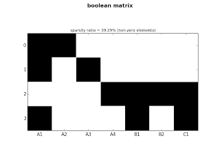
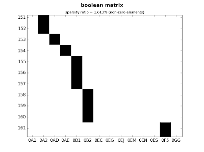
Let's plot both matrices used on the previous examples:
    ct.plot_sparse(ticks=True, x_ticks=True, sparsity=True)
    
fig.1: small matrix
    ct.plot_sparse(ticks=False, sparsity=True)
    
fig.2: medium matrix
    ct.plot_sparse(ticks=True, x_ticks=True, sparsity=True)
    
fig.3: medium matrix - detail
That's all for this post, I hope you find it useful.